
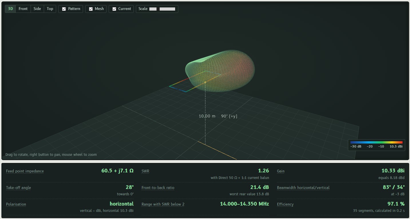
Rudolf Schuba, DA6BOC, published a web-based antenna simulator Antennenrechner, which is used without registration and without installation. The tool is developed exclusively from open-source components and may be used free of charge. The current version at the time of preparation of the article is 1.8.0-beta from October 11, 2026. The author expressly points out that he does not guarantee the correctness of the calculations: the results must be verified before construction and the antenna tuned at the installation site.
The practical value of the tool lies in the shorter journey from idea to drawing. Instead of local installation of 4nec2 or EZNEC and manually writing the cards, just select the antenna type, band and press the Starting values button. The result is also a finished construction plan in PDF.
You will read in the article
Computing core and architecture
The simulation runs on nec2c, which is a C translation of the original NEC-2 code from Lawrence Livermore National Laboratory (N. Kyriazis, version 1.3.1, GPL-3.0). This is the method of moments, the same as in the well-known programs for wire antennas. According to the 1.0.0-beta release, nec2c runs in a Docker container and the nec2c source code is part of the application as a standalone program.
| Component | The task | Version |
|---|---|---|
| no2c | computing core NEC-2 | 1.3.1 |
| Python | server | 3.12.15 |
| Starlette, Uvicorn | web framework and server | 1.7.0, 0.54.0 |
| NumPy, SciPy | numerics, optimizer, interpolation | 2.5.4, 1.18.1 |
| three.js | 3D display in the browser | r170 |
| Matplotlib, ReportLab | charts and PDF generation | 3.11.2, 5.0.1 |
From the point of view of operation, it is interesting that all libraries and fonts are provided from the own server, without external services. As of version 1.2.0, the application has security headers including Content-Security-Policy, a limit on the number of requests per IP address, and is designed to run behind a reverse proxy. The limit of one calculation is 120 s and the maximum size of the model is 1500 segments. For large antennas with many additional bands or high frequencies, a longer calculation time must therefore be expected.
Supported antenna types and frequency range
There is a choice of dipole (including inverted V and Windom), EFHW and long wire, ground plane, yagi, Moxon, Delta loop, quad and free geometry of any wires. Models from other programs (Help mentions 4nec2 and EZNEC) are imported from .nec files and the current model is also exported. The project is saved as a *.antenne.json file on the local disk; nothing is stored on the server.

Since version 1.6.0, microwave bands of 13 cm, 9 cm, 6 cm, 3 cm and 1.2 cm and frequencies up to 30 GHz have been added. From 1 GHz, the construction plan lists dimensions in millimeters with a resolution of 0.01 mm. At these frequencies, instead of ferrite transformers, a sleeve balun or direct coaxial feeding is used.

A parabolic antenna (version 1.7.0) is not calculated in NEC-2, but according to aperture theory, because the reflector is many wavelengths in diameter. The diameter and f/D ratio are entered, or in the case of an existing parabola, the depth measured in the center from the plane of the edge, from which f/D is calculated. This is practical when adjusting the satellite dish. Can (circular waveguide), patch or helix for circular polarization can be chosen as the irradiator. The output is gain, beamwidth, first sidelobe, efficiency breakdown and edge taper. Offset parabolas are currently approximated by a rotationally symmetric parabola of the same aperture, so it is only an estimate.
Trimming and optimization

After the calculation, the length is fine-tuned with the Trim to resonance function, which adjusts the length or circumference to resonance; at the Yagi to adjust with hairpins. Optimise is also available for Yagi, Moxon and quad, which improves gain and front-to-back ratio. It runs in free space and lasts up to approximately 30 seconds. Optimizing without the influence of the ground is a compromise: the result for an antenna at a low height above the ground may differ, and after optimization it is advisable to make a new calculation with a real ground model.
The earth model is selected automatically. The demanding Sommerfeld calculation is used only for antennas lower than 0.2 λ, above this height the approximation via the reflection coefficient is used, while the difference is less than 1.5 Ω according to the author.
Resonances tab
Broadband sweep, by default from 0.4 to 3.5 times the center frequency, displays SWR and impedance curves with amateur bands highlighted. Series resonances (X = 0, low impedance) are indicated by a solid triangle, parallel (X = 0, high impedance, typical of EFHW) by an empty one. The findings are in a table and in a PDF. Help gives an example of when this is useful: whether a dipole for 10 m is also usable for 6 m or 4 m.
Customization and baluns
In Automatic mode, the program selects the variant with the best SWR: direct supply, balun or Unun, λ/4 line or hairpin. The range of transformations is 1:1 to 64:1. The Matching tab lists the SWR for each option and data for winding or lead length. The author states that the data for winding baluns and ununs are common practical values from radio amateur practice. With multiband antennas (EFHW, long wire, Windom), additional bands can be evaluated via the band buttons. Each additional band is calculated as a separate, appropriately segmented model.
The initial dimensions of the Moxon are based on the approximate formulas of L. B. Cebik, W4RNL, and the Yagi boom length correction is based on the approximation according to DL6WU.
Interface
The appearance is reminiscent of a measuring instrument: a panel with 3D display, graphs and data, band buttons with indicator lights and the B612 font designed by Airbus and Intactile for cockpit displays. Interface, Info and PDF pages switch between German and English. Concepts with dotted underlining are explained in the tooltip (on touch screens, tap) and the same explanation is in the Legend tab.
In the 3D view, it rotates with the left mouse button, pans with the right and zooms with the wheel. The radiation diagram has a color scale from −30 dB (blue) to maximum (red), optionally also coloring the wires according to the current. It is the current distribution across the elements that is useful in diagnosing why a Yagi or quad is behaving differently than expected. SWR up to 1.5 is green, usable yellow and high red. In addition, the program gives gain in both dBi and dBd, peak elevation angle (low for DX, steep for NVIS), front-to-back ratio, beamwidth in −3 dB, and frequency range with SWR below 2.
Construction plan in PDF
The Build plan PDF button creates a document with key simulation data, a 3D view image at the right angle, a dimensional sketch, tables of model and cut lengths (for Yagi, the lengths and spacing of all elements), a list of materials and construction notes. It also includes recommended fitting, SWR and impedance curves, diagrams and possibly a band overview and resonance table. In the case of a parabola, a profile will be added as a rib template and the dimensions of the irradiator. The choice of conductor insulation affects only the cut lengths: the insulated wire is cut slightly shorter. If the inputs have changed since the last calculation, the PDF will be recalculated automatically before creation.
Limitations and recommendations
The simulation assumes a free environment. Poles, buildings, trees, power cable and the actual ground all shift resonance and impedance. The author recommends building antennas 2 to 5% longer and tuning them at the resulting location to minimum SWR. Help also warns that after each change of frequency you have to press Starting values again.
The change history also shows the practical benefit of the feedback: version 1.5.1 fixed a bug where the EFHW and long wire power point in the model was up to 1.25 m below the specified height (8.75 instead of 10 m at 80 m); error reported by DL2HXA. For long wires, therefore, consider a recalculation for older calculations.
For an important project, it makes sense to export the model to a .nec file and compare the result in another program that reads this format, for example in 4nec2.